The Sustainability of State & Local Pensions: A Public Finance Approach

Introduction

State and local government pension plans are important economic institutions in the United States. They hold nearly $5 trillion in assets; their annual payments to beneficiaries are equal to about 1.5 percent of national GDP; and over 11 million beneficiaries rely on these payments to support themselves in retirement. In recent years, attention has focused on the plans’ large unfunded liabilities and the need to fully fund these obligations. But is full funding the only way to achieve fiscal sustainability?

This brief, which is based on a recent paper, explores an alternative path to the fiscal sustainability of state and local pension plans – namely, stabilizing their pension debt as a share of the economy.¹Lenney et al. (2021). To assess the feasibility of this approach requires: 1) projecting the annual cash flows for a nationally-representative sample of 40 state and local pension systems to see the future evolution of each plan under current contribution levels; and 2) estimating the contribution increases needed to stabilize the ratio of pension debt to the economy.

The discussion proceeds as follows. The first section provides background on the fiscal stability of state and local plans. The second section describes the data and methodology. The third section presents the results for when plans will exhaust their assets under current funding levels and benefit provisions. A key finding is that pension benefits, as a share of the economy, are currently near their peak and will decline significantly over time due to the reforms instituted by many plans. Nevertheless, many plans are at risk over the long term of exhausting their assets, so action will be needed. The fourth section presents the results on the alternative path, specifically the contribution changes required to stabilize pension debt, both in the long run and to get the ratio at the end of 30 years back to today’s level.

The final section concludes that the United States is not facing a state and local pension crisis but, over the longer term, a large share of plans face the risk of insolvency. Hence, they would need to increase contributions to achieve sustainability. But the required adjustments to stabilize debt relative to the economy are generally moderate in size and, in all cases, substantially lower than the adjustments required under the typical full prefunding framework.

Background

In recent years, public pension analysts have focused intensely on the need for full prefunding of state and local pensions. The approach would enable a plan to shut down at any time and pay full benefits without additional contributions. This emphasis on full funding is a relatively new development. As recently as 2008, many analysts considered a funding ratio of 80 percent to be sound practice for state and local plans.²U.S. Government Accountability Office (2008). But academics and policymakers have embraced the full funding goal with gusto.

In academic work, some researchers explicitly state that full prefunding is the proper goal for plans,³Boyd and Yin (2016). while others make the argument implicitly by focusing analysis on the fiscal costs of transitioning to full funding.⁴Novy-Marx and Rauh (2014). With regard to policymakers, CalPERS, the nation’s largest state and local pension plan, explicitly advocates for full funding, stating that the “ideal level” of prefunding is 100 percent.⁵California Public Employees’ Retirement System (2014). Along similar lines, a blue ribbon panel commissioned by the Society of Actuaries “wholeheartedly believes that…plans should be pre-funded.”⁶Society of Actuaries (2014). Finally, ratings agencies typically view “underfunding of pension…benefits as [a] key credit issue.”⁷S&P Global Ratings (2019).

Yet, full prefunding is not the only way to make a pension system sustainable.⁸Indeed, the theoretical literature on optimal pension funding is decidedly mixed in its conclusions. For example, tax smoothing considerations may dictate a wide range of optimal funding levels, including levels substantially below full funding, depending on economic conditions (D’Arcy, Dulebohn, and Oh 1999). If most voters are borrowers and government borrowing costs are lower than voters’ borrowing costs, then no prefunding is optimal in many instances (Bohn 2011). Furthermore, to the extent that state and local government expenditures are investments (e.g., schooling) rather than consumption, borrowing is appropriate as the benefits from that spending accrue in the future (Sheiner 2021).

Other papers focus on the costs of not prefunding: asymmetric information between government employees and other voters over the cost of pensions may allow government workers to accrue rents in the absence of prefunding (Bagchi 2019 and Glaeser and Ponzetto 2014); and unfunded pensions may lower the capital stock (Feldstein 1974). Finally, Lucas (2017) provides a thorough discussion of both the uncertainty surrounding optimal funding levels for state and local pensions, as well as arguments for and against full funding. Indeed, even an unfunded pay-as-you-go program with a dedicated income stream – such as Social Security – can honor obligations without recourse to additional funding as long as the internal rate of return paid to beneficiaries does not exceed the growth rate of the wage base.⁹Samuelson (1958). Of course, pay-as-you-go programs can face shortfalls if demographic changes increase the growth in outlays or lower the growth of revenues. However, mature, partially funded systems, such as state and local pension plans, which have accumulated assets to provide a buffer, can remain sustainable even in the face of adverse shocks.

More broadly, unfunded pension liabilities are simply a form of government debt. Such public debt can be sustainable as long as the government makes appropriate service payments on it. The requirement for holding pension debt stable relative to the economy depends on the relationship between the growth rate of the economy (g) and the interest rate (r). If r = g, then the required annual contribution to the pension fund is simply the normal cost – the cost of benefits accrued in a given year. When the rate of interest is greater than the growth rate of the economy, r > g, contributions have to be sufficient to cover the normal cost and debt service costs. If r < g, then debt can be held constant as a share of the economy with contributions less than the normal cost. While the required contribution rate is dependent on the assumed relationship between r and g, the key point is that sustainability does not require full funding – stabilizing pension debt as a share of the economy should allow the government to meet all its pension obligations without crowding out other public services.

Moreover, transitioning to full funding involves generational transfers – with current generations paying higher taxes/having lower benefits in order to reduce taxes/raise benefits on future generations. Stabilizing the level of funding is a way of equalizing burdens across generations.

Data and Methodology

The basis for the analysis is projecting the future flow of benefits for state and local pension plans. The principal source for these calculations is the Public Plans Database (PPD) maintained by the Center for Retirement Research at Boston College. The PPD contains plan-level data accounting for 95 percent of state and local plan membership and assets in the United States. This analysis uses a sample of 40 plans, which includes the largest 20 public pension plans and an additional 20 selected so that the sample matches the national PPD sample in terms of funding, budgetary, and demographic characteristics.

For the individual state and local plans in the sample, additional information comes from the plan’s actuarial valuations and the state’s Comprehensive Annual Financial Reports for FY 2017.¹⁰Specifically, these publications provide data on: 1) the age and service distribution of currently employed members (actives); 2) average salaries by age and service for the currently employed members; 3) the age distribution of current beneficiaries; 4) the distribution of average benefits for current beneficiaries by age; 5) mortality assumptions by status (active employee or beneficiary); 6) termination rates by age and service; and 7) retirement rates by age and service and plan tier. The reports also include plan provisions and actuarial assumptions not available in the PPD: the plan benefit factor, normal retirement age, early retirement age, service requirement, vesting requirement, salary averaging method, penalty factor for early retirement (percentage reduction per year early), plan marriage and spousal benefit assumptions, gender ratio of the active employee population, and cost-of-living adjustment (COLA) assumptions.

Annual pension benefits are typically equal to the years of service multiplied by final average salary times the benefit factor. Thus, the benefit factor is the percentage of final salary to which a pension beneficiary is entitled for each year of service. Typically, the average salary from the highest three to five years is used to determine the final salary.

The methodology can be divided into three stages. The first stage involves estimating the future flow of benefit payments to current beneficiaries and workers. This process requires using mortality tables to age the initial distribution of current beneficiaries each year and information about their pension benefits by age to calculate annual benefit payments. For current workers, the process involves aging the workforce each year (incrementing years of service and age) and using the probabilities of retirement, disability, death, and quits or termination by age and years of service to create a matrix of new beneficiaries by year. Information on pension eligibility, benefit formulas, and economic assumptions is then used to calculate the pension obligations for these new beneficiaries by year.¹¹These benefit formulas vary by plan tier to capture the effects of reforms implemented between cohorts of active workers. Projections are checked against the liabilities reported in the relevant actuarial valuations. Then, the cash flows are re-estimated using consistent economic assumptions – nominal wage growth of 3.4 percent and CPI inflation of 2.2 percent. Although these procedures are conceptually quite straightforward, the actual implementation is very complex.

The second stage involves projecting plan membership growth to estimate benefits for future workers. New hires in each year are set equal to the previous year’s head count multiplied by the sum of the projected growth rate in the government’s workforce and the proportion of withdrawals and retirements from the workforce in the previous year. Projected workforce growth keeps constant the ratio of the government workforce to the working-age population. A further assumption is that the age distribution and relative salaries of new hires match the distribution of current employees with fewer than five years of service. Each group of new hires then produces a new stream of benefits starting at each future year, with the value of those future benefits calculated in exactly the same way as they were for the current active workers but adjusting for changes to plan provisions instituted for new hires.

The final stage requires pairing the benefit cash flow projections with information on asset levels and assumed future returns to assess the fiscal outlook for each plan. For plan assets, the starting point is PPD data for FY 2017, but asset values changed significantly between FY 2017 and FY 2021, so the values are updated for our analysis.¹²The asset valuations are updated in three steps: benchmarking to the plan’s most recent financial report; after that, applying returns on appropriate indexes to update to February 2021; and finally, applying assumed general returns to grow assets from February 2021 to the end of the fiscal year. On average, the calculations indicate that plan assets increased 23 percent from the end of FY 2017 to the end of FY 2021.

Since then, after we completed the study on which this brief is based, aggregate plan assets have fallen about 20 percent, which aligns with the roughly 20-percent drop in equities over the same period. Lower asset levels make acheiving any funding goal (e.g. full prefunding or stabilizing pension debt as a share of the economy) harder.

To calculate future asset levels, the analysis assumes three alternative real rates of return.

• The lowest – 0.5 percent – is roughly equal to the longer-run risk-free rate in recent years, as reflected by the yield on the zero-coupon 20-year Treasury Inflation Projected Securities.
• The intermediate assumption – 2.5 percent – is equivalent to the return on a mixed portfolio containing 60 percent risk-free assets and 40 percent equities.
• The highest – 4.5 percent – reflects the expected return on a pension portfolio comprised of 20 percent risk-free assets and 80 percent equities.

An important issue is whether investment returns on pension assets should be risk-adjusted in government budget projections. Such an adjustment would prevent plans from appearing healthier simply because they invest in riskier assets. This issue is difficult and contentious. The Congressional Budget Office, for example, uses a risk-free rate of return for programs like student loans in its “Fair Value” approach, but uses expected returns in its budget accounting.

In all cases, plan liabilities in this analysis are calculated by discounting promised benefits by the 0.5-percent real risk-free rate. This approach incorporates the assumption that pension obligations will be paid out in full in nearly all future states of the world. This assumption is unlikely to be strictly true, which makes it conservative.¹³In particular, most pension plans have the legal ability to change the COLA even for existing retirees. In any case, the results are not very sensitive to the chosen discount rate because the focus is the stability of pension debt rather than its level. In contrast, exercises that calculate what is required for plans to be fully funded are very sensitive to the assumed discount rate on liabilities.

Results: Outlook with Current Contributions

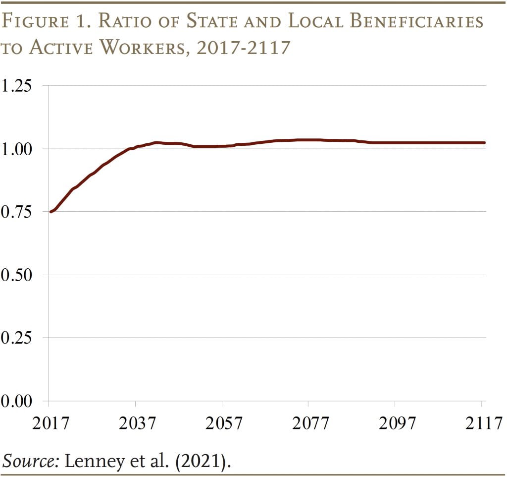
The projections produced four major findings. The first is that the ratio of beneficiaries to workers in state and local governments is projected to increase about 36 percent from 2017 to 2040 and then roughly stabilize (see Figure 1). This finding is consistent with projections by the Social Security actuaries, which show that the ratio of Social Security beneficiaries to workers is projected to rise about 39 percent over this time period.¹⁴These calculations refer to data for federal retirement and disability benefits (U.S. Social Security Administration 2020). This comparison is appropriate because state and local pensions also cover disability as well as retirement. This similarity offers some support that the future flow of state and local government employees has been appropriately modeled.

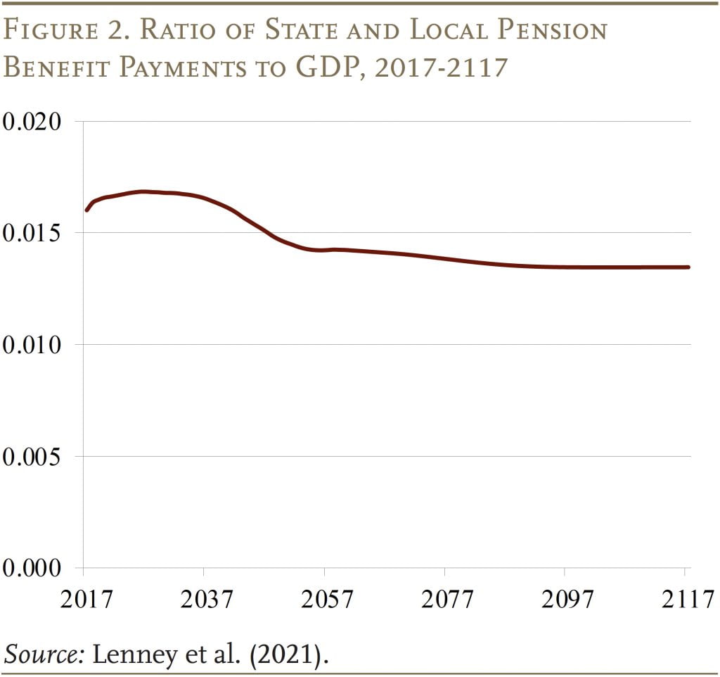
The second finding is that, despite the rising ratio of beneficiaries to workers, annual benefit payments as a share of the economy is already near its peak (see Figure 2). This surprising result can be attributed to two factors. First, most pension plans do not fully index their retiree benefits for inflation, which lowers the real value of average benefits over time. Second, pension plans have gradually been making changes to lower benefits and raise retirement ages for new hires.¹⁵Aubry and Crawford (2017). The reduced growth in average benefits due to the COLA restraints and new hire reforms offsets a large share of the effects of the 36-percent growth in the ratio of beneficiaries to workers.

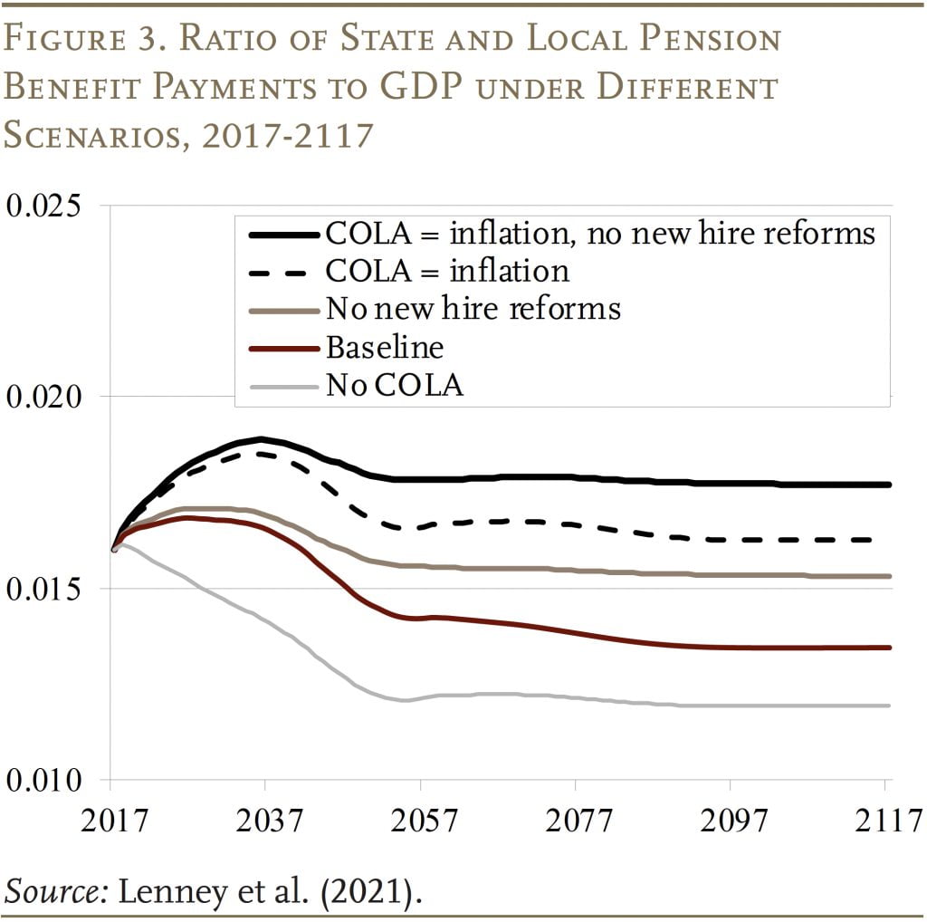
To drive the point home regarding the discrepancy between the pattern for beneficiaries/workers and benefits/GDP, Figure 3 documents the impact of changing assumptions about COLAs and new hire reforms. The top line, which assumes a full COLA and no benefit reductions for new hires, shows the same rising pattern evident in the ratio of beneficiaries to workers. Subsequent lines show the impact of incorporating the new hire reforms into the projections.

The fact that pension benefits as a share of payroll are, in aggregate, near their highest level expected over the next few decades is an important finding for understanding the sustainability of state and local finances and the ability of plans to smooth through this period.

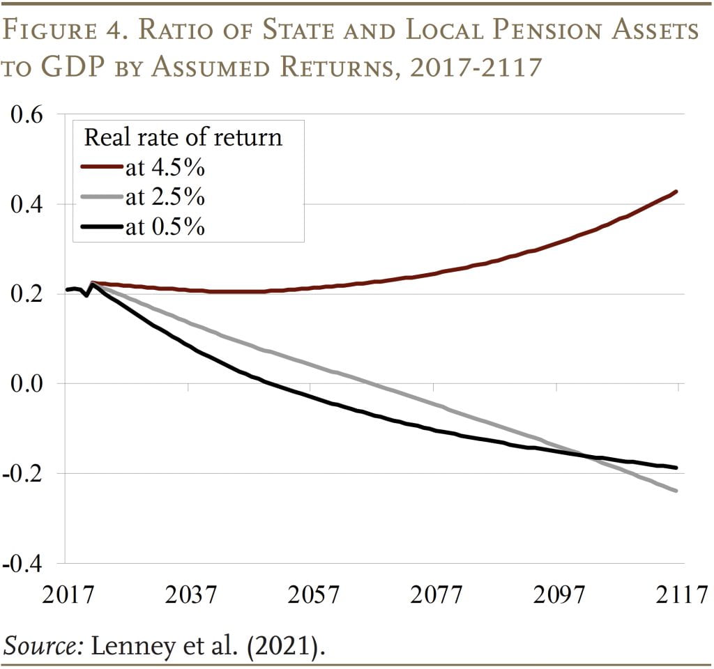
The third finding in this current policy analysis pertains to the paths for assets, relative to the economy, under the three asset return assumptions (see Figure 4). Summing across the plans, with the 0.5-percent real rate of return, current contributions are insufficient to keep the plans solvent. Despite the projected decline in benefits relative to GDP, assets relative to GDP begin declining immediately and are exhausted in about 30 years. With a 2.5-percent rate of return, assets are declining, but not as quickly; they are exhausted in 47 years. In contrast, if plans earn 4.5 percent on their assets, they are sustainable: at current contribution rates, assets rise indefinitely and the plans face no fiscal stress.

Of course, looking at the exhaustion of pension assets for the system as a whole masks a lot of variation across plans. Figure 5 shows the share of liabilities in plans that exhaust within various time periods. With a 0.5-percent real rate of return, about 6 percent of liabilities are in plans that exhaust within 20 years and 43 percent are in plans that exhaust within 30 years; even at this low rate of return, 23 percent of liabilities are in plans that never exhaust. At a 2.5-percent real return, only 7 percent of liabilities are in plans that exhaust within the next 30 years, and 38 percent are in plans that never exhaust. With a 4.5-percent real return, almost 60 percent of liabilities are in plans that never exhaust, whereas the other plans do exhaust, but mostly not for many decades.¹⁶One notable exception is the New Jersey Teacher’s Plan, which exhausts in 10 years even with a rate of return of 4.5 percent.

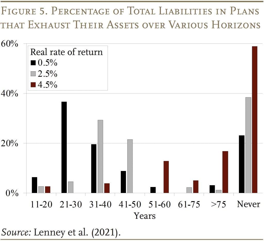
The message from these exercises is that the majority of plans do not face an imminent crisis in the sense that they are likely to exhaust their assets within the next two decades. But a sizeable share could exhaust their assets within 30 years under the low-return scenario. And even under the high-return scenario, more than 40 percent are at risk of depleting their assets over longer time horizons. Thus, adjustments will be necessary. The questions are: How large are those adjustments? and How urgent are they?

Results: Pension Debt Stabilization

This analysis involves estimating the changes in pension contributions required to stabilize pension debt relative to GDP. The first exercise asks what permanent changes in the contribution rate would make pension debt eventually stabilize as a share of GDP. Because very long-run projections are inherently uncertain, the second exercise asks what permanent changes in contributions would get debt as a share of GDP back to today’s level in 30 years.¹⁷The first exercise stabilizes the debt-to-GDP ratio without specifying a target level, which does not account for potential changes in borrowing costs that might arise if the ultimate debt-to-GDP ratio were higher than it is today – for example, due to credit rating downgrades. The second exercise eliminates this concern by picking today’s ratio as the target.

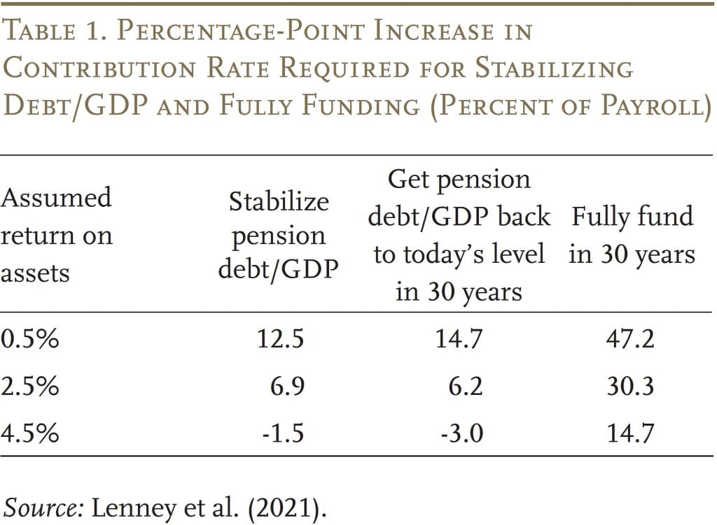
The results of the simulations are shown in Table 1. The required increase in the contribution rate to stabilize the debt-to-GDP ratio is 12.5 percentage points when assets yield 0.5 percent; 6.9 percentage points with a return of 2.5 percent; and contributions could be cut with a return of 4.5 percent.¹⁸One possibility is that plans could run out of assets along the way, which might be a constraint, both economically and politically (see Costrell and McGee 2020). In the aggregate, under a 2.5-percent-return scenario, assets do decline but they never approach zero. That said, some individual plans do exhaust their assets, at which point the simulations assume these governments issue marketable debt – akin to a pension obligation bond to fund benefits – and thereafter make service payments on the marketable debt. The numbers look very similar with a goal of getting the debt/GDP ratio back to today’s level in 30 years. To put these contribution changes into context, aggregate pension contributions increased by 10 percentage points between 2009 and 2019.¹⁹Based on the full PPD sample, updated through FY 2019. The final column shows that the required percentage-point increase in contribution rates to fully fund these plans would be four or five times larger. Of course, looking at results for the entire state and local pension system hides substantial variation among plans (see Appendix).

The analysis also produces some surprising results. First, acting sooner rather than later lowers the required increase, but not by much. For example, assuming assets earn a real rate of return of 2.5 percent, even if the plans do nothing for 30 years, the required increase only rises from 6.9 percent to 8.6 percent of payroll. When rates of return are assumed to be very low – specifically, less than the growth rate of the economy – the contributions required to stabilize the debt are, of course, higher. But, strikingly, under this scenario, it is also true that acting sooner rather than later doesn’t help. The intuition here is that when interest rates are less than the growth rate of the economy, government debt has no fiscal costs.²⁰See Blanchard (2019). When r < g, holding more assets is costly because they constantly shrink as a share of the economy; thus, running down assets and then beginning the stabilization process later allows stabilization with a lower contribution rate compared to starting sooner. If, instead, r = g or r > g, failing to act early would raise the required increase in the contribution rate.

The second surprising finding is that the poorly funded plans are not the ones that have to make the greatest contributions to stabilize. The reason is that these poorly funded plans have increased their contribution rates significantly, made the largest cuts to benefits for new hires, and reduced their COLAs. Plans that made the largest changes in contributions since 2007 and the biggest reforms to their benefits are currently contributing more than enough to stabilize their debt, even at a 0.5-percent rate of return in many cases.

Conclusion

This brief started by exploring the fiscal outlook for state and local government pension plans under current benefit and funding policies. The projections show no sign of a massive pension crisis in the next two decades. In fact, despite the projected increase in the ratio of beneficiaries to workers, benefit payments as a share of the economy are currently near their peak and will eventually decline significantly. As a result, these plans can be put on a sustainable footing – by stabilizing the ratio of pension debt to the economy – with contribution rate increases roughly equal to those adopted over the last 20 years.

Shifting the focus to achieving sustainability by maintaining a stable debt-to-GDP ratio from the more typical emphasis on full prefunding merits serious consideration. In an effort to prefund, state and local governments have increased their pension contributions dramatically over the past 20 years. These increased contributions come at a significant opportunity cost. Despite the long economic expansion that preceded the brief COVID recession, provision of public goods provided by state and local governments remained depressed: real per capita spending on infrastructure stood at about 25 percent below its previous peak, and state and local government employment per capita also remained well below its previous peak. Notably, much of this relative decline in state and local government employment occurred in the K-12 and higher education sectors.

The research summarized in this brief is certainly not the last word on the topic. Indeed, other researchers have critiqued various aspects of the analysis.²¹Rauh (2021) and Lucas (2021). But, continuing with status quo or increasingly stringent full-funding policies also has costs. So, hopefully the basic idea presented here is a first step towards building a more sustainable framework for managing state and local pension plan liabilities.

References

Aubry, Jean-Pierre and Caroline V. Crawford. 2017. “State and Local Pension Reform since the Financial Crisis.” State and Local Plans Issue in Brief 54. Chestnut Hill, MA: Center for Retirement Research at Boston College.

Bagchi, Sutirtha. 2019. “The Effects of Political Competition on the Generosity of Public-Sector Pension Plans.” Journal of Economic Behavior and Organization 164: 439-468.

Blanchard, Olivier. 2019. “Public Debt and Low Interest Rates.” American Economic Review 109(4): 1197-229.

Bohn, Henning. 2011. “Should Public Retirement Plans Be Fully Funded?” Journal of Pension Economics and Finance 10(2): 195-219.

Boyd, Donald J. and Yimeng Yin. 2016. “Public Pension Funding Practices.” Albany, NY: Nelson A. Rockefeller Institute of Government.

California Public Employees’ Retirement System. 2014. Annual Review of Funding Levels and Risks, 2014. Sacramento, CA.

Costrell, Robert M. and Josh McGee. 2020. “Sins of the Past, Present, and Future: Alternative Pension Funding Policies.” Paper prepared for the Municipal Finance Conference (July 13-14). Washington, DC: Brookings Institution, Hutchins Center on Fiscal and Monetary Policy.

D’Arcy, Stephen P., James H. Dulebohn, and Pyungsuk Oh. 1999. “Optimal Funding of State Employee Pension Systems.” Journal of Risk and Insurance 66(3): 345-380.

Feldstein, Martin. 1974. “Social Security, Induced Retirement, and Aggregate Capital Accumulation.” Journal of Political Economy 82(5): 905-926.

Glaeser, Edward L. and Giacomo A. M. Ponzetto. 2014. “Shrouded Costs of Government: The Political Economy of State and Local Public Pensions.” Journal of Public Economics 116: 89-105.

Lenney, Jamie, Byron Lutz, Finn Schüle, and Louise Sheiner. 2021. “The Sustainability of State and Local Pensions: A Public Finance Approach.” Brookings Papers on Economic Activity (Spring): 1-48.

Lucas, Deborah J. 2017. “Towards Fair Value Accounting for Public Pensions: The Case for Delinking Disclosure and Funding Requirements.” Prepared for Gathering Storm: The Risks of State Pension Underfunding Conference (October 19-20). Cambridge, MA: Harvard Kennedy School.  Citations are to an unpublished 2020 version.

Lucas, Deborah. 2021. “Comments and General Discussion of ‘The Sustainability of State and Local Pensions: A Public Finance Approach.’” Brookings Papers on Economic Activity (Spring): 49-57.

Novy-Marx, Robert and Joshua D. Rauh. 2014. “Linking Benefits to Investment Performance in US Public Pension Systems.” Journal of Public Economics 116:47–61.

Public Plans Database. 2001-2021. Center for Retirement Research at Boston College, MissionSquare Research Institute, National Association of State Retirement Administrators, and Government Finance Officers Association.

Rauh, Joshua. 2021. “Comments and General Discussion of ‘The Sustainability of State and Local Pensions: A Public Finance Approach.’” Brookings Papers on Economic Activity (Spring): 57-63.

Samuelson, Paul A. 1958. “An Exact Consumption-Loan Model of Interest with or without the Social Contrivance of Money.” Journal of Political Economy 66(6): 467-482.

Sheiner, Louise. 2021. “What Debt Crisis? Time to Stop Worrying and Spend What’s Needed to Fix the Economy.” Milken Institute Review. Available at:

Society of Actuaries. 2014. Blue Ribbon Panel on Public Pension Plan Funding. Schaumberg, IL.

S&P Global Ratings. 2019. “U.S. Public Finance 2018 Year in Review.” New York, NY.

U.S. Government Accountability Office (GAO). 2008. State and Local Government Retiree Benefits: Current Funded Status of Pension and Health Benefits. Washington, DC.

U.S. Social Security Administration. 2020. The Annual Reports of the Board of Trustees of the Federal Old-Age and Survivors Insurance and Federal Disability Insurance Trust Funds.Washington, DC: U.S. Government Printing Office.

Appendix

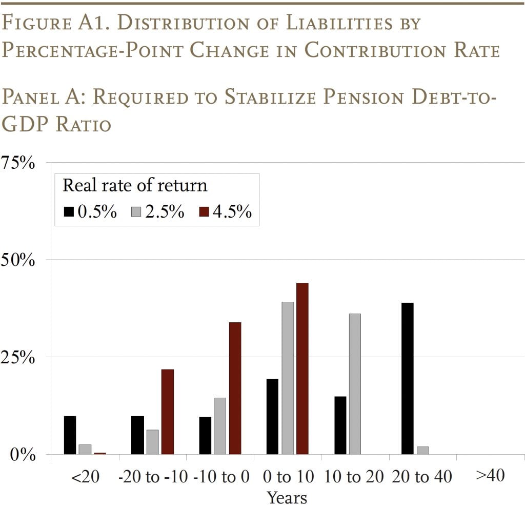
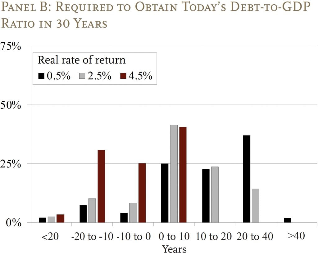
The required increase in contribution rates to fully fund state and local plans varies substantially among plans. Panel A of Figure A1 shows the distribution of required adjustments for plans to stabilize the debt over the long run starting immediately. For example, at the 2.5-percent rate of return, only 2 percent of liabilities are in plans that need to increase funding by more than 20 percent of payroll, and less than 40 percent of liabilities are in plans where the contribution increase is more than 10 percent of payroll. At a 0.5-percent return, however, 39 percent need to increase contributions by more than 20 percent of payroll. Panel B shows the changes required to obtain today’s debt-to-GDP ratio in 30 years, and the results look quite similar.

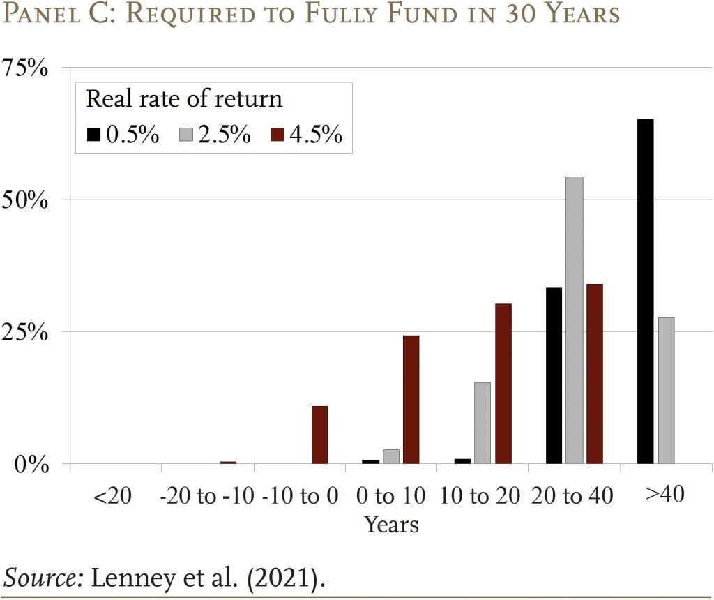
Finally, Panel C, which presents the distribution of required contribution changes to fully fund the plans, shows most of the liabilities are in plans that require at least a 20-percentage-point increase in the rate, and even if plans earn 4.5 percent on their assets, they will have to make a substantial increase in their contribution rates.

Endnotes

• 1
  Lenney et al. (2021).
• 2
  U.S. Government Accountability Office (2008).
• 3
  Boyd and Yin (2016).
• 4
  Novy-Marx and Rauh (2014).
• 5
  California Public Employees’ Retirement System (2014).
• 6
  Society of Actuaries (2014).
• 7
  S&P Global Ratings (2019).
• 8
  Indeed, the theoretical literature on optimal pension funding is decidedly mixed in its conclusions. For example, tax smoothing considerations may dictate a wide range of optimal funding levels, including levels substantially below full funding, depending on economic conditions (D’Arcy, Dulebohn, and Oh 1999). If most voters are borrowers and government borrowing costs are lower than voters’ borrowing costs, then no prefunding is optimal in many instances (Bohn 2011). Furthermore, to the extent that state and local government expenditures are investments (e.g., schooling) rather than consumption, borrowing is appropriate as the benefits from that spending accrue in the future (Sheiner 2021).
  
  Other papers focus on the costs of not prefunding: asymmetric information between government employees and other voters over the cost of pensions may allow government workers to accrue rents in the absence of prefunding (Bagchi 2019 and Glaeser and Ponzetto 2014); and unfunded pensions may lower the capital stock (Feldstein 1974). Finally, Lucas (2017) provides a thorough discussion of both the uncertainty surrounding optimal funding levels for state and local pensions, as well as arguments for and against full funding.
• 9
  Samuelson (1958).
• 10
  Specifically, these publications provide data on: 1) the age and service distribution of currently employed members (actives); 2) average salaries by age and service for the currently employed members; 3) the age distribution of current beneficiaries; 4) the distribution of average benefits for current beneficiaries by age; 5) mortality assumptions by status (active employee or beneficiary); 6) termination rates by age and service; and 7) retirement rates by age and service and plan tier. The reports also include plan provisions and actuarial assumptions not available in the PPD: the plan benefit factor, normal retirement age, early retirement age, service requirement, vesting requirement, salary averaging method, penalty factor for early retirement (percentage reduction per year early), plan marriage and spousal benefit assumptions, gender ratio of the active employee population, and cost-of-living adjustment (COLA) assumptions.
  
  Annual pension benefits are typically equal to the years of service multiplied by final average salary times the benefit factor. Thus, the benefit factor is the percentage of final salary to which a pension beneficiary is entitled for each year of service. Typically, the average salary from the highest three to five years is used to determine the final salary.
• 11
  These benefit formulas vary by plan tier to capture the effects of reforms implemented between cohorts of active workers.
• 12
  The asset valuations are updated in three steps: benchmarking to the plan’s most recent financial report; after that, applying returns on appropriate indexes to update to February 2021; and finally, applying assumed general returns to grow assets from February 2021 to the end of the fiscal year. On average, the calculations indicate that plan assets increased 23 percent from the end of FY 2017 to the end of FY 2021.
  
  Since then, after we completed the study on which this brief is based, aggregate plan assets have fallen about 20 percent, which aligns with the roughly 20-percent drop in equities over the same period. Lower asset levels make acheiving any funding goal (e.g. full prefunding or stabilizing pension debt as a share of the economy) harder.
• 13
  In particular, most pension plans have the legal ability to change the COLA even for existing retirees.
• 14
  These calculations refer to data for federal retirement and disability benefits (U.S. Social Security Administration 2020). This comparison is appropriate because state and local pensions also cover disability as well as retirement.
• 15
  Aubry and Crawford (2017).
• 16
  One notable exception is the New Jersey Teacher’s Plan, which exhausts in 10 years even with a rate of return of 4.5 percent.
• 17
  The first exercise stabilizes the debt-to-GDP ratio without specifying a target level, which does not account for potential changes in borrowing costs that might arise if the ultimate debt-to-GDP ratio were higher than it is today – for example, due to credit rating downgrades. The second exercise eliminates this concern by picking today’s ratio as the target.
• 18
  One possibility is that plans could run out of assets along the way, which might be a constraint, both economically and politically (see Costrell and McGee 2020). In the aggregate, under a 2.5-percent-return scenario, assets do decline but they never approach zero. That said, some individual plans do exhaust their assets, at which point the simulations assume these governments issue marketable debt – akin to a pension obligation bond to fund benefits – and thereafter make service payments on the marketable debt.
• 19
  Based on the full PPD sample, updated through FY 2019.
• 20
  See Blanchard (2019). When r < g, holding more assets is costly because they constantly shrink as a share of the economy; thus, running down assets and then beginning the stabilization process later allows stabilization with a lower contribution rate compared to starting sooner. If, instead, r = g or r > g, failing to act early would raise the required increase in the contribution rate.
• 21
  Rauh (2021) and Lucas (2021).