How Does Local Cost-of-Living Affect Retirement?

Introduction

Households across the United States face very different cost-of-living, largely due to variations in housing expenses. Over the last 50 years, house prices have risen fastest in already expensive areas. To attract workers despite high prices, these local labor markets offer more wages and/or fringe benefits. Wage levels directly affect retirement security through Social Security benefits, which, by design, replace a higher share of pre-retirement earnings for workers at the bottom of the national earnings distribution, not taking local price levels into account. As a result, households in high-cost areas could face a replacement-rate penalty if their employers offer higher wages. The questions are: 1) How large is this penalty in practice? and 2) Do workers respond to the penalty by adjusting their behavior?

This brief, based on a recent paper, uses the Health and Retirement Study to document the relationship between local cost-of-living – captured by housing prices – and Social Security replacement rates.¹Quinby and Wettstein (2022). It then explores whether households in high-cost areas compensate for lower replacement rates by responding in three possible ways: saving more during their working years; retiring later; and/or moving to a lower-cost area when they retire.

The discussion proceeds as follows. The first section provides background on the link between local cost-of-living and Social Security replacement rates. The second section describes the data and methodology. The third section presents results for the association between local cost-of-living, replacement rates, and household behavior. The final section concludes that Social Security replacement rates are lower in more-expensive areas, but the gap is somewhat smaller than anticipated because earnings have only partially kept up with the cost of financing a house. In response to the gap that does exist, households – especially the more educated – save more; and some homeowners move after retirement.

Background

Most U.S. households spend a large share of their budget on housing – around 40 percent, on average.²Klick and Stockberger (2021). The next largest budget items are food and transportation (each about 15 percent). Consequently, when they decide where to live and work, they often factor in house prices. Over the last 50 years, constraints on the supply of housing in coastal labor markets, such as the metro areas of New York City and San Francisco, have caused prices to rise faster than the national average.³Saiz (2010); Van Nieuwerburgh and Weill (2010); and Gyourko, Mayer, and Sinai (2013). As a result, employers in these high-cost labor markets pay more to attract and retain workers.⁴Rosen (1979); Roback (1982); and Ganong and Shaog (2017).

This higher compensation could put households at a disadvantage when it comes to retirement income. Social Security calculates retirement benefits based on a national formula that is a progressive function of workers’ lifetime earnings. If high-cost labor markets pay higher wages to compensate, then workers in these areas receive lower Social Security replacement rates than otherwise identical workers in low-cost labor markets.

Such a replacement-rate penalty could impact households’ saving, labor supply, and location decisions. First, households in expensive locations could save more in 401(k)s to compensate for low Social Security replacement rates.⁵Of course, homeowners in expensive locations automatically build wealth through their house. However, this study focuses on saving in employer-sponsored retirement plans as well as other financial accounts because few retired households tap their home equity to support daily consumption (Poterba, Venti, and Wise 2011). Enhanced home equity could also crowd out other forms of saving. Second, workers might delay retirement to enhance their monthly Social Security benefits – to take advantage of the actuarial adjustment for later claiming, give their savings more time to grow, and shorten the period over which their savings need to stretch.⁶The actuarial adjustment increases monthly benefits for each month of later claiming to hold lifetime benefits roughly constant for a person with average life expectancy. Lastly, retired households could live more economically in retirement by moving to a lower-cost location. The question is whether geographic variation in replacement rates is large enough to induce these types of responses.

Data and Methodology

Data for the analysis come primarily from the Health and Retirement Study (HRS), a nationally representative longitudinal survey of older households that has been fielded every two years between 1992 and 2020. The sample includes households who have agreed to link their public survey data with lifetime earnings records from the Social Security Administration.⁷Earnings data are linked for about two thirds of the full HRS sample, and are currently available through 2018. In some instances when administrative earnings data are unavailable, it is possible to estimate the respondent’s lifetime earnings history using self-reports about the timing and duration of past jobs. Households are observed when the highest lifetime earner – measured by Social Security’s Average Indexed Monthly Earnings (AIME) – is age 55 or 56 (depending on the two-year HRS interval).⁸AIME is a measure of lifetime earnings used by the Social Security Administration to calculate retirement and disability benefits. AIME is determined by first adjusting annual earnings to account for real wage growth in the economy over time. Then, the highest 35 years of indexed earnings are averaged (and divided by 12) to produce AIME. In this brief, we examine households’ annualized AIME, which sums the individual AIME of the household head and spouse, then multiplies by 12.

HRS data on where people live are used to link retirees with their local housing market. The focus here is Metropolitan Statistical Areas (MSAs), which capture major population centers and their suburbs. The American Community Survey (ACS) provides data on housing prices across MSAs from 2005 onward. To impute house prices in earlier years, the Federal Housing Finance Agency calculates a price index for MSAs from 1992-2005 that can be applied to the ACS data. In addition, the ACS and the Current Population Survey provide data that are used to control for the strength of the local economy.
The first stage of the analysis uses a regression to establish the relationship between local house prices and Social Security replacement rates:

Replacement rate = ƒ(log median house price in the household’s MSA, household characteristics,
local labor demand)

The outcome variable is the share of the household’s lifetime earnings replaced by Social Security benefits, if claimed at the full retirement age. The independent variable of interest is the median house price in the household’s MSA. If house prices drive up wages as predicted (driving down the replacement rate), then the coefficient on this variable will be negative and statistically significant. Household characteristics include standard demographic and socio-economic factors. Local labor demand is captured by the prime-age employment rate in the household’s MSA.

The analysis then turns to behavioral impacts. The regression analysis described above is adapted to include three new outcomes of interest: 1) a measure of saving, defined as the household’s financial assets divided by lifetime earnings; 2) the Social Security claiming age anticipated by the household’s highest earner; and 3) an indicator for moving to a different MSA.⁹The moving variable reflects the probability of relocating to a different MSA before the highest earner turns age 70.

Results

This section summarizes the two sets of results; first, for how cost-of-living variations affect Social Security replacement rates and, second, for households’ behavioral responses.

How Much Does Cost-of-Living Affect Social Security Benefits?

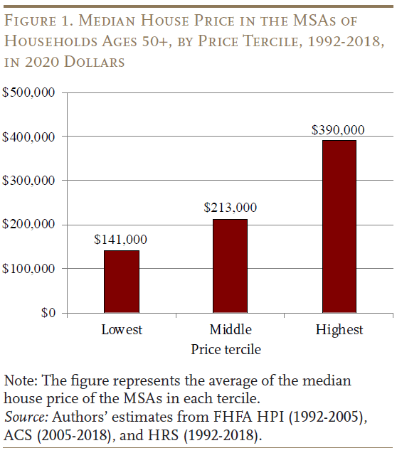
To provide context for the analysis, Figure 1 contrasts the typical median house price, in 2020 dollars, for households in low, medium, and high-cost areas between 1992 and 2018. These housing cost terciles are obtained by ranking the national population by the median house price in their MSA and then dividing the population into thirds.¹⁰The ranking includes both renters and homeowners because rents are assumed to fully reflect the local price of housing. Figure 1 shows that households in the bottom two terciles experience relatively similar housing prices, whereas those in the top tercile face prices that are around double.

The next question is how much a household’s earnings would need to rise to fully offset the difference in housing costs. To get a rough sense, we consider what households in 1992-2018 would have paid – on average – to finance the purchase of a house in the lowest price tercile.¹¹This back-of-the-envelope estimate assumes a fixed 30-year loan with 10 percent down, a 6-percent interest rate (Federal Reserve Bank of St Louis 2022), and a credit score of 700 (DeNicola 2022). The calculation uses the online mortgage calculator provided by bankrate.com. We then compare that mortgage payment to what households would have paid for a house in the highest price tercile. This exercise suggests that earnings need to rise about 32 percent, between the bottom and the top terciles, to fully offset the cost of housing.

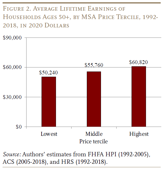
Yet, Figure 2 shows only a 20-percent increase in average household earnings between the bottom and top price terciles: $50,000 compared to $61,000.¹²Figure 2 defines earnings in terms of AIME. The gap between housing-cost growth and earnings is even more stark within education groups. Comparing earnings across price terciles separately for those with and without a college degree shows only a 13-percent increase from the bottom to the top terciles. The difference is due to households’ location decisions – highly educated households tend to locate in more expensive MSAs, driving up average earnings in the third price tercile. These numbers suggest that older households are only partly compensated for local housing costs, at least in terms of wages.¹³This finding is consistent with Ganong and Shoag (2017).

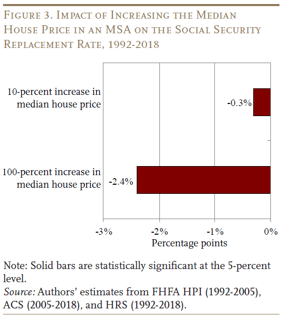
Not surprisingly, then, regression results for the relationship between Social Security replacement rates and local house prices show only a modest effect (see Figure 3). Controlling for household characteristics, a 10-percent increase in the median house price in a household’s MSA is only associated with a 0.3 percentage-point decrease in the replacement rate. Even doubling the median house price is only associated with a 2.4-percentage-point decrease in the replacement rate. Although this relationship is highly statistically significant, it is economically small given that the average replacement rate in the lowest-cost MSAs is 53 percent.

Do Households Respond to Local Cost-of-Living?

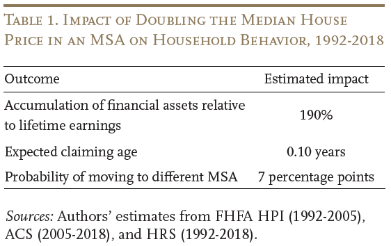
The next phase of the analysis considers how households respond to local cost-of-living. Table 1 presents regression estimates for the three outcomes of interest: 1) savings, measured as financial assets relative to household earnings; 2) expected claiming age; and 3) the probability of moving.

On the saving front, doubling the median house price in a household’s MSA is associated with increased financial assets worth nearly two times lifetime average annual earnings. This amount of new saving virtually eliminates the replacement-rate gap. For example, in 2021, households in the highest-cost MSAs could use their additional savings to purchase an annuity on the private market that, when combined with Social Security, would replace around 53 percent of their lifetime earnings. This 53-percent replacement rate is equal to what households in lower-cost MSAs get from Social Security.¹⁴Households in the high-cost MSAs earn $61,000 in lifetime earnings on average (see Figure 3), implying a monthly Social Security benefit of $2,440 and additional savings of just under $115,000 (1.87*$61,000=$114,070). These savings could be used to purchase a private annuity yielding around $260 per month, bringing total monthly income to about $2,700 ($2,440 plus a $260 private annuity). This total monthly income replaces 53 percent of lifetime earnings ($2,700 *12/$61,000). The private annuity calculation assumes a 100-percent joint and survivor annuity (paying the same benefit so long as either spouse is still living) with a 3-percent COLA for a 65-year-old man and his 60-year-old wife. The price quote was obtained from Annuity Shopper archives (available at https://www.immediateannuities.com/pdfs/as/annuity-shopper-2021-01.pdf).

Turning to the claiming age, the impact of the median house price is positive – indicating that workers retire later when they live in high-cost areas, all else equal – but it is small in magnitude and statistically insignificant.

Finally, with respect to decisions about relocating, Table 1 shows that households living in high-cost areas are more likely to move across MSAs, but the regression estimate is only weakly significant. It turns out that moving is highly dependent on homeownership status, with homeowners in high-cost areas more likely to move than renters living in those same areas (see Figure 4).¹⁵The sample size of renters is too small to rule out substantial effects.

Conclusion

Across the country, workers with similar skills earn different compensation to reflect the cost of housing in their local labor market. Yet, Social Security benefits are determined by a national formula that does not take local price levels into account. To the extent that living in an area with a high cost-of-living translates to higher wages, workers in these areas could end up with lower replacement rates than otherwise similar workers in less-expensive areas. If the difference is substantial, workers might respond by saving more, working longer, or retiring to a lower-cost location.

The results of this analysis show that Social Security replacement rates are lower in more-expensive areas, but the gap is somewhat smaller than anticipated because earnings have only partially kept up with the cost of financing a house. In response to the gap that does exist, households – especially the more educated – save more; and some homeowners move when they retire.

References

DeNicola, Louis. 2022. “What is a Good Credit Score?” Costa Mesa, CA: Experian. Available at: https://www.experian.com/blogs/ask-experian/credit-education/score-basics/what-is-a-good-credit-score/

Federal Housing Finance Agency. House Price Index, 1992-2005. Washington, DC.

Federal Reserve Bank of St Louis. 2022. “30-Year Fixed Rate Mortgage Average in the United States.” St. Louis, MO. Available at: https://fred.stlouisfed.org/series/MORTGAGE30US

Ganong, Peter and Daniel Shoag. 2017. “Why Has Regional Income Convergence in the U.S. Declined?” Journal of Urban Economics 102: 76-90.

Gyourko, Joseph, Christopher Mayer, and Todd Sinai. 2013. “Superstar Cities.” American Economic Journal: Economic Policy 5(4): 167-199.

Klick, Josh and Anya Stockberger. 2021. “Experimental CPI for Lower and Higher Income Households.” Working Paper 537. Washington, DC: U.S. Bureau of Labor Statistics.

Poterba, James, Steven Venti, and David Wise. 2011. “The Composition and Drawdown of Wealth in Retirement.” Journal of Economic Perspectives 25(4): 95-118.

Quinby, Laura D. and Gal Wettstein. 2022. “How Does Local Cost-of-Living Affect Retirement?” Working Paper 2022-15. Chestnut Hill, MA: Center for Retirement Research at Boston College.

Roback, Jennifer. 1982. “Wages, Rents, and the Quality of Life.” Journal of Political Economy 90(6): 1257-1278.

Rosen, Harvey S. 1979. “Housing Decisions and the U.S. Income Tax: An Econometric Analysis.” Journal of Public Economics 11(1): 1-23.

Saiz, Albert. 2010. “The Geographic Determinants of Housing Supply.” The Quarterly Journal of Economics 125(3): 1253-1296.

University of Michigan. Health and Retirement Study, 1992-2018. Ann Arbor, MI.

U.S. Census Bureau. American Community Survey, 2005-2018. Washington, DC.

Van Nieuwerburgh, Stijn and Pierre-Olivier Weill. 2010. “Why Has House Price Dispersion Gone Up?” The Review of Economic Studies 77(4): 1567-1606.

Endnotes

• 1
  Quinby and Wettstein (2022).
• 2
  Klick and Stockberger (2021). The next largest budget items are food and transportation (each about 15 percent).
• 3
  Saiz (2010); Van Nieuwerburgh and Weill (2010); and Gyourko, Mayer, and Sinai (2013).
• 4
  Rosen (1979); Roback (1982); and Ganong and Shaog (2017).
• 5
  Of course, homeowners in expensive locations automatically build wealth through their house. However, this study focuses on saving in employer-sponsored retirement plans as well as other financial accounts because few retired households tap their home equity to support daily consumption (Poterba, Venti, and Wise 2011). Enhanced home equity could also crowd out other forms of saving.
• 6
  The actuarial adjustment increases monthly benefits for each month of later claiming to hold lifetime benefits roughly constant for a person with average life expectancy.
• 7
  Earnings data are linked for about two thirds of the full HRS sample, and are currently available through 2018. In some instances when administrative earnings data are unavailable, it is possible to estimate the respondent’s lifetime earnings history using self-reports about the timing and duration of past jobs.
• 8
  AIME is a measure of lifetime earnings used by the Social Security Administration to calculate retirement and disability benefits. AIME is determined by first adjusting annual earnings to account for real wage growth in the economy over time. Then, the highest 35 years of indexed earnings are averaged (and divided by 12) to produce AIME. In this brief, we examine households’ annualized AIME, which sums the individual AIME of the household head and spouse, then multiplies by 12.
• 9
  The moving variable reflects the probability of relocating to a different MSA before the highest earner turns age 70.
• 10
  The ranking includes both renters and homeowners because rents are assumed to fully reflect the local price of housing.
• 11
  This back-of-the-envelope estimate assumes a fixed 30-year loan with 10 percent down, a 6-percent interest rate (Federal Reserve Bank of St Louis 2022), and a credit score of 700 (DeNicola 2022). The calculation uses the online mortgage calculator provided by bankrate.com.
• 12
  Figure 2 defines earnings in terms of AIME. The gap between housing-cost growth and earnings is even more stark within education groups. Comparing earnings across price terciles separately for those with and without a college degree shows only a 13-percent increase from the bottom to the top terciles. The difference is due to households’ location decisions – highly educated households tend to locate in more expensive MSAs, driving up average earnings in the third price tercile.
• 13
  This finding is consistent with Ganong and Shoag (2017).
• 14
  Households in the high-cost MSAs earn $61,000 in lifetime earnings on average (see Figure 3), implying a monthly Social Security benefit of $2,440 and additional savings of just under $115,000 (1.87*$61,000=$114,070). These savings could be used to purchase a private annuity yielding around $260 per month, bringing total monthly income to about $2,700 ($2,440 plus a $260 private annuity). This total monthly income replaces 53 percent of lifetime earnings ($2,700 *12/$61,000). The private annuity calculation assumes a 100-percent joint and survivor annuity (paying the same benefit so long as either spouse is still living) with a 3-percent COLA for a 65-year-old man and his 60-year-old wife. The price quote was obtained from Annuity Shopper archives (available at https://www.immediateannuities.com/pdfs/as/annuity-shopper-2021-01.pdf).
• 15
  The sample size of renters is too small to rule out substantial effects.